Axis

Creating an Axis

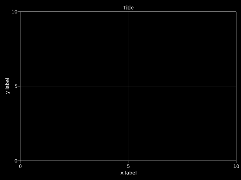
The Axis is a 2D axis that works well with automatic layouts. Here's how you create one

using CairoMakie

f = Figure()

ax = Axis(f[1, 1], xlabel = "x label", ylabel = "y label",
    title = "Title")

f

Plotting into an Axis

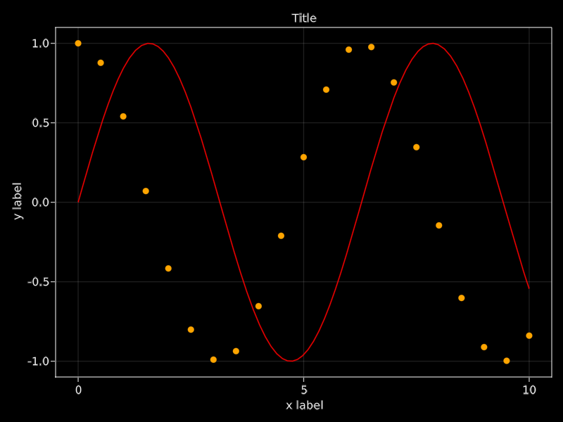
You can use all the normal mutating 2D plotting functions with an Axis. These functions return the created plot object. Omitting the ax argument plots into the current_axis(), which is usually the axis that was last created.

lineobject = lines!(ax, 0..10, sin, color = :red)
scatobject = scatter!(0:0.5:10, cos, color = :orange)

f

Deleting plots

You can delete a plot object directly via delete!(ax, plotobj). You can also remove all plots with empty!(ax).

using CairoMakie

f = Figure()

axs = [Axis(f[1, i]) for i in 1:3]

scatters = map(axs) do ax
    [scatter!(ax, 0:0.1:10, x -> sin(x) + i) for i in 1:3]
end

delete!(axs[2], scatters[2][2])
empty!(axs[3])

f

Setting Axis limits and reversing axes

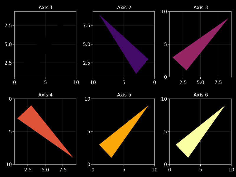
You can set axis limits with the functions xlims!, ylims! or limits!. The numbers are meant in the order left right for xlims!, and bottom top for ylims!. Therefore, if the second number is smaller than the first, the respective axis will reverse. You can manually reverse an axis by setting ax.xreversed = true or ax.yreversed = true.

Note that if you enforce an aspect ratio between x-axis and y-axis using autolimitaspect, the values you set with these functions will probably not be exactly what you get, but they will be changed to fit the chosen ratio.

using CairoMakie

f = Figure()

axes = [Axis(f[i, j]) for j in 1:3, i in 1:2]

for (i, ax) in enumerate(axes)
    ax.title = "Axis $i"
    poly!(ax, Point2f[(9, 9), (3, 1), (1, 3)],
        color = cgrad(:inferno, 6, categorical = true)[i])
end

xlims!(axes[1], [0, 10]) # as vector
xlims!(axes[2], 10, 0) # separate, reversed
ylims!(axes[3], 0, 10) # separate
ylims!(axes[4], (10, 0)) # as tuple, reversed
limits!(axes[5], 0, 10, 0, 10) # x1, x2, y1, y2
limits!(axes[6], BBox(0, 10, 0, 10)) # as rectangle

f

Setting half-automatic limits

You can set half limits by either giving one argument as nothing or by using the keyword syntax where only low or high is given.

using CairoMakie

f = Figure()

data = rand(100, 2) .* 0.7 .+ 0.15

Axis(f[1, 1], title = "xlims!(nothing, 1)")
scatter!(data)
xlims!(nothing, 1)

Axis(f[1, 2], title = "xlims!(low = 0)")
scatter!(data)
xlims!(low = 0)

Axis(f[2, 1], title = "ylims!(0, nothing)")
scatter!(data)
ylims!(0, nothing)

Axis(f[2, 2], title = "ylims!(high = 1)")
scatter!(data)
ylims!(high = 1)

f

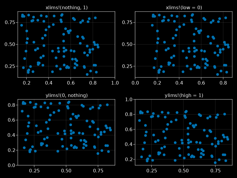
This also works when specifying limits directly, such as Axis(..., limits = (nothing, 1, 2, nothing)).

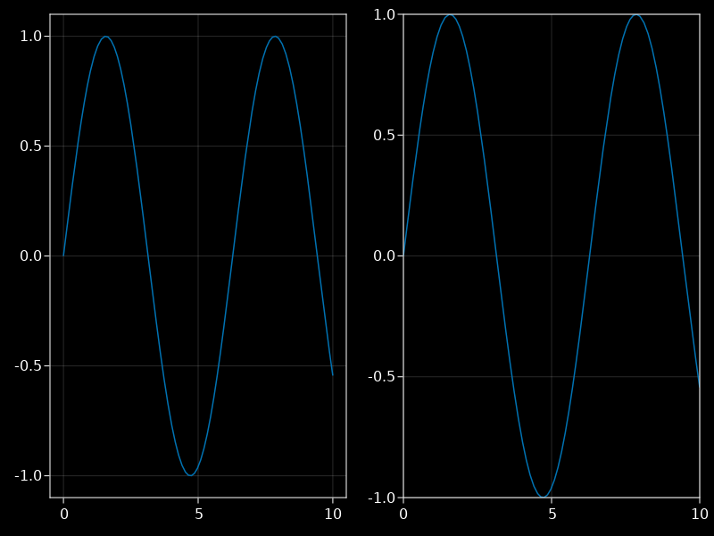
Auto-reset behavior

When you create a new plot in an axis, reset_limits!(ax) is called, which adjusts the limits to the new bounds. If you have previously set limits with limits!, xlims! or ylims!, these limits are not overridden by the new plot. If you want to override the manually set limits, call autolimits!(ax) to compute completely new limits from the axis content.

The user-defined limits are stored in ax.limits. This can either be a tuple with two entries, where each entry can be either nothing or a tuple with numbers (low, high).It can also be a tuple with four numbers (xlow, xhigh, ylow, yhigh). You can pass this directly when creating a new axis. The same observable limits is also set using limits!, xlims! and ylims!, or reset to (nothing, nothing) using autolimits!.

using CairoMakie

f = Figure()

lines(f[1, 1], 0..10, sin)
lines(f[1, 2], 0..10, sin, axis = (limits = (0, 10, -1, 1),))

f

Modifying ticks

To control ticks, you can set the axis attributes xticks/yticks and xtickformat/ytickformat.

You can overload one or more of these three functions to implement custom ticks:

tickvalues, ticklabels = MakieLayout.get_ticks(ticks, scale, formatter, vmin, vmax)
tickvalues = MakieLayout.get_tickvalues(ticks, vmin, vmax)
ticklabels = MakieLayout.get_ticklabels(formatter, tickvalues)

If you overload get_ticks, you have to compute both tickvalues and ticklabels directly as a vector of floats and strings, respectively. Otherwise the result of get_tickvalues is passed to get_ticklabels by default. The limits of the respective axis are passed as vmin and vmax.

A couple of behaviors are implemented by default. You can specify static ticks by passing an iterable of numbers. You can also pass a tuple with tick values and tick labels directly, bypassing the formatting step.

As a third option you can pass a function taking minimum and maximum axis value as arguments and returning either a vector of tickvalues which are then passed to the current formatter, or a tuple with tickvalues and ticklabels which are then used directly.

For formatting, you can pass a function which takes a vector of numbers and outputs a vector of strings. You can also pass a format string which is passed to Formatting.format from Formatting.jl, where you can mix the formatted numbers with other text like in "{:.2f}ms".

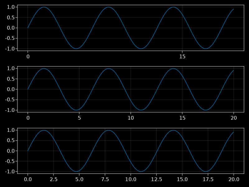
Predefined ticks

The default tick type is LinearTicks(n), where n is the target number of ticks which the algorithm tries to return.

using CairoMakie

fig = Figure()
for (i, n) in enumerate([2, 5, 9])
    lines(fig[i, 1], 0..20, sin, axis = (xticks = LinearTicks(n),))
end
fig

There's also WilkinsonTicks which uses the alternative Wilkinson algorithm.

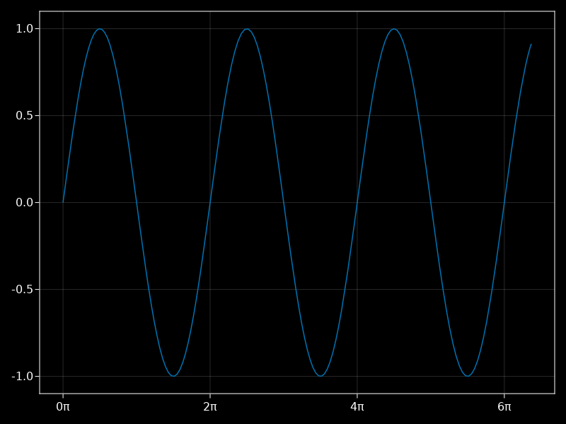
MultiplesTicks can be used when an axis should be marked at multiples of a certain number. A common scenario is plotting a trigonometric function which should be marked at pi intervals.

using CairoMakie

lines(0..20, sin, axis = (xticks = MultiplesTicks(4, pi, "π"),))

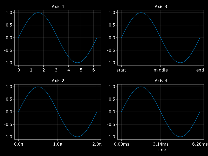
Here are a couple of examples that show off different settings for ticks and formats.

using CairoMakie

f = Figure()

axes = [Axis(f[i, j]) for i in 1:2, j in 1:2]

xs = LinRange(0, 2pi, 50)
for (i, ax) in enumerate(axes)
    ax.title = "Axis $i"
    lines!(ax, xs, sin.(xs))
end

axes[1].xticks = 0:6

axes[2].xticks = 0:pi:2pi
axes[2].xtickformat = xs -> ["$(x/pi)π" for x in xs]

axes[3].xticks = (0:pi:2pi, ["start", "middle", "end"])

axes[4].xticks = 0:pi:2pi
axes[4].xtickformat = "{:.2f}ms"
axes[4].xlabel = "Time"

f

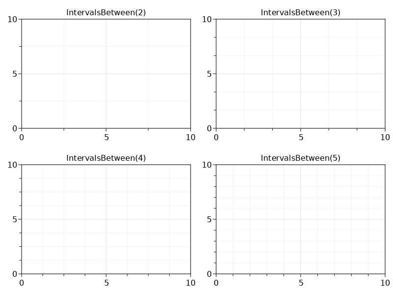
Minor ticks and grids

You can show minor ticks and grids by setting x/yminorticksvisible = true and x/yminorgridvisible = true which are off by default. You can set size, color, width, align etc. like for the normal ticks, but there are no labels. The x/yminorticks attributes control how minor ticks are computed given major ticks and axis limits. For that purpose you can create your own minortick type and overload MakieLayout.get_minor_tickvalues(minorticks, tickvalues, vmin, vmax).

The default minor tick type is IntervalsBetween(n, mirror = true) where n gives the number of intervals each gap between major ticks is divided into with minor ticks, and mirror decides if outside of the major ticks there are more minor ticks with the same intervals as the adjacent gaps.

using CairoMakie

theme = Attributes(
    Axis = (
        xminorticksvisible = true,
        yminorticksvisible = true,
        xminorgridvisible = true,
        yminorgridvisible = true,
    )
)

fig = with_theme(theme) do
    fig = Figure()
    axs = [Axis(fig[fldmod1(n, 2)...],
        title = "IntervalsBetween($(n+1))",
        xminorticks = IntervalsBetween(n+1),
        yminorticks = IntervalsBetween(n+1)) for n in 1:4]
    fig
end

fig

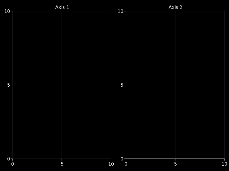
Hiding Axis spines and decorations

You can hide all axis elements manually, by setting their specific visibility attributes to false, like xticklabelsvisible, but that can be tedious. There are a couple of convenience functions for this.

To hide spines, you can use hidespines!.

using CairoMakie

f = Figure()

ax1 = Axis(f[1, 1], title = "Axis 1")
ax2 = Axis(f[1, 2], title = "Axis 2")

hidespines!(ax1)
hidespines!(ax2, :t, :r) # only top and right

f

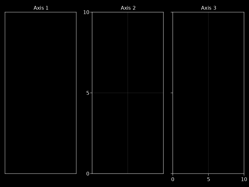
To hide decorations, you can use hidedecorations!, or the specific hidexdecorations! and hideydecorations!. When hiding, you can set label = false, ticklabels = false, ticks = false, grid = false, minorgrid = false or minorticks = false as keyword arguments if you want to keep those elements. It's common, e.g., to hide everything but the grid lines in facet plots.

using CairoMakie

f = Figure()

ax1 = Axis(f[1, 1], title = "Axis 1")
ax2 = Axis(f[1, 2], title = "Axis 2")
ax3 = Axis(f[1, 3], title = "Axis 3")

hidedecorations!(ax1)
hidexdecorations!(ax2, grid = false)
hideydecorations!(ax3, ticks = false)

f

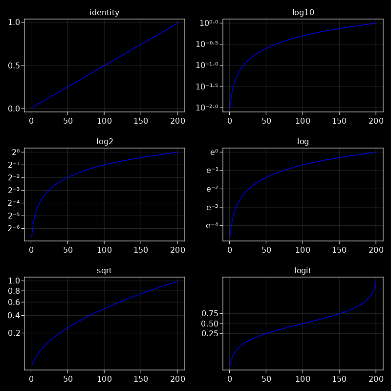
Log scales and other axis scales

The two attributes xscale and yscale, which by default are set to identity, can be used to project the data in a nonlinear way, in addition to the linear zoom that the limits provide.

Take care that the axis limits always stay inside the limits appropriate for the chosen scaling function, for example, log functions fail for values x <= 0, sqrt for x < 0, etc.

using CairoMakie

data = LinRange(0.01, 0.99, 200)

f = Figure(resolution = (800, 800))

for (i, scale) in enumerate([identity, log10, log2, log, sqrt, Makie.logit])

    row, col = fldmod1(i, 2)
    Axis(f[row, col], yscale = scale, title = string(scale),
        yminorticksvisible = true, yminorgridvisible = true,
        yminorticks = IntervalsBetween(8))

    lines!(data, color = :blue)
end

f

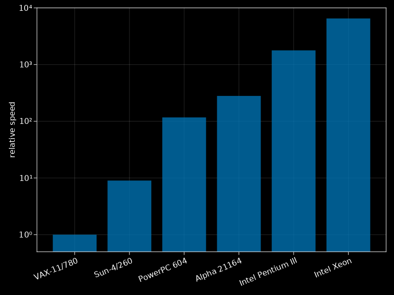
Pseudolog and symlog scales

Some plotting functions, like barplots or density plots, have offset parameters which are usually zero, which you have to set to some non-zero value explicitly so they work in log axes.

using CairoMakie

processors = ["VAX-11/780", "Sun-4/260", "PowerPC 604",
    "Alpha 21164", "Intel Pentium III", "Intel Xeon"]
relative_speeds = [1, 9, 117, 280, 1779, 6505]

barplot(relative_speeds, fillto = 0.5,
    axis = (yscale = log10, ylabel ="relative speed",
        xticks = (1:6, processors), xticklabelrotation = pi/8))

ylims!(0.5, 10000)
current_figure()

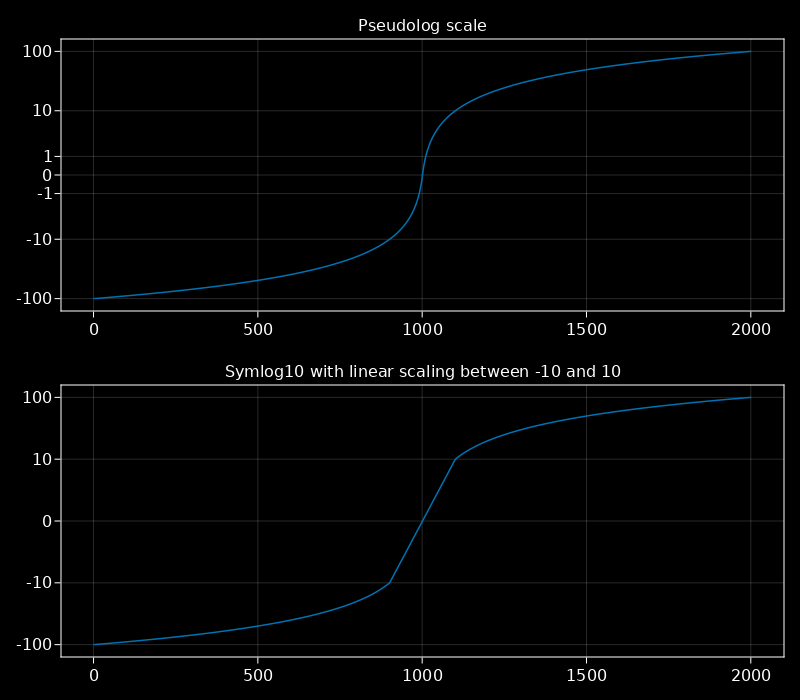
Another option are pseudolog and symlog scales. Pseudolog is similar to log, but modified in order to work for zero and for negative values. The pseudolog10 function is defined as sign(x) * log10(abs(x) + 1).

Another option for symmetric log scales including zero is the symmetric log scale Symlog10, which combines a normal log scale with a linear scale between two boundary values around zero.

using CairoMakie

f = Figure(resolution = (800, 700))

lines(f[1, 1], -100:0.1:100, axis = (
    yscale = Makie.pseudolog10,
    title = "Pseudolog scale",
    yticks = [-100, -10, -1, 0, 1, 10, 100]))

lines(f[2, 1], -100:0.1:100, axis = (
    yscale = Makie.Symlog10(10.0),
    title = "Symlog10 with linear scaling between -10 and 10",
    yticks = [-100, -10, 0, 10, 100]))

f

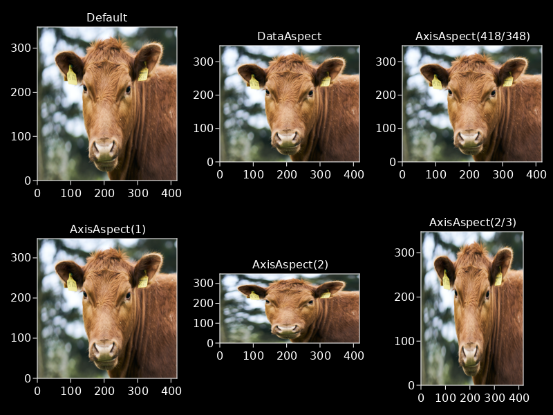
Controlling Axis aspect ratios

If you're plotting images, you might want to force a specific aspect ratio of an axis, so that the images are not stretched. The default is that an axis uses all of the available space in the layout. You can use AxisAspect and DataAspect to control the aspect ratio. For example, AxisAspect(1) forces a square axis and AxisAspect(2) results in a rectangle with a width of two times the height. DataAspect uses the currently chosen axis limits and brings the axes into the same aspect ratio. This is the easiest to use with images. A different aspect ratio can only reduce the axis space that is being used, also it necessarily has to break the layout a little bit.

using CairoMakie
using FileIO

f = Figure()

axes = [Axis(f[i, j]) for i in 1:2, j in 1:3]
tightlimits!.(axes)

img = rotr90(load(assetpath("cow.png")))

for ax in axes
    image!(ax, img)
end

axes[1, 1].title = "Default"

axes[1, 2].title = "DataAspect"
axes[1, 2].aspect = DataAspect()

axes[1, 3].title = "AxisAspect(418/348)"
axes[1, 3].aspect = AxisAspect(418/348)

axes[2, 1].title = "AxisAspect(1)"
axes[2, 1].aspect = AxisAspect(1)

axes[2, 2].title = "AxisAspect(2)"
axes[2, 2].aspect = AxisAspect(2)

axes[2, 3].title = "AxisAspect(2/3)"
axes[2, 3].aspect = AxisAspect(2/3)

f

Controlling data aspect ratios

If you want the content of an axis to adhere to a certain data aspect ratio, there is another way than forcing the aspect ratio of the whole axis to be the same, and possibly breaking the layout. This works via the axis attribute autolimitaspect. It can either be set to nothing which means the data limits can have any arbitrary aspect ratio. Or it can be set to a number, in which case the targeted limits of the axis (that are computed by autolimits!) are enlarged to have the correct aspect ratio.

You can see the different ways to get a plot with an unstretched circle, using different ways of setting aspect ratios, in the following example.

using CairoMakie
using Animations



# scene setup for animation
###########################################################

container_scene = Scene(camera = campixel!, resolution = (1200, 1200))

t = Node(0.0)

a_width = Animation([1, 7], [1200.0, 800], sineio(n=2, yoyo=true, postwait=0.5))
a_height = Animation([2.5, 8.5], [1200.0, 800], sineio(n=2, yoyo=true, postwait=0.5))

scene_area = lift(t) do t
    Recti(0, 0, round(Int, a_width(t)), round(Int, a_height(t)))
end

scene = Scene(container_scene, scene_area, camera = campixel!)

rect = poly!(scene, scene_area,
    raw=true, color=RGBf(0.97, 0.97, 0.97), strokecolor=:transparent, strokewidth=0)

outer_layout = GridLayout(scene, alignmode = Outside(30))




# example begins here
###########################################################

layout = outer_layout[1, 1] = GridLayout()

titles = ["aspect enforced\nvia layout", "axis aspect\nset directly", "no aspect enforced", "data aspect conforms\nto axis size"]
axs = layout[1:2, 1:2] = [Axis(scene, title = t) for t in titles]

for a in axs
    lines!(a, Circle(Point2f(0, 0), 100f0))
end

rowsize!(layout, 1, Fixed(400))
# force the layout cell [1, 1] to be square
colsize!(layout, 1, Aspect(1, 1))

axs[2].aspect = 1
axs[4].autolimitaspect = 1

rects = layout[1:2, 1:2] = [Box(scene, color = (:black, 0.05),
    strokecolor = :transparent) for _ in 1:4]

record(container_scene, joinpath(@OUTPUT, "example_circle_aspect_ratios.mp4"), 0:1/30:9; framerate=30) do ti
    t[] = ti
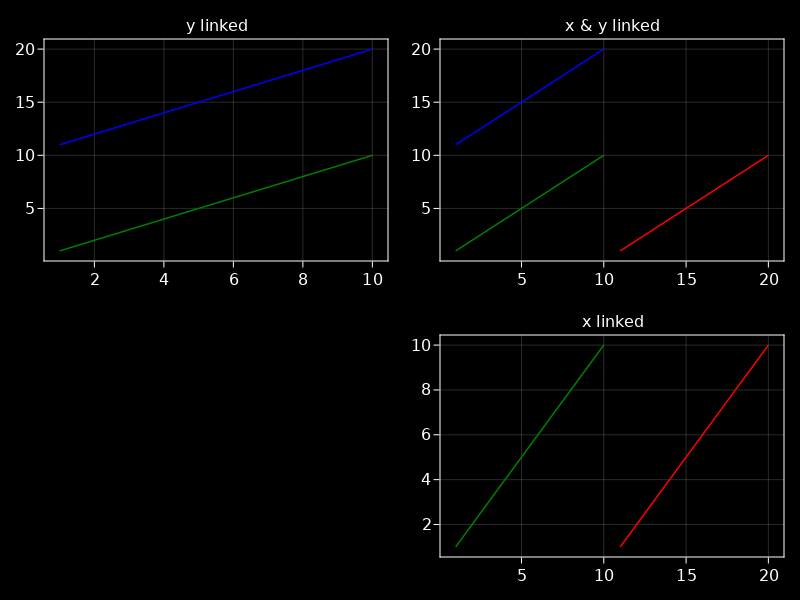
end

Linking axes

You can link axes to each other. Every axis simply keeps track of a list of other axes which it updates when it is changed itself. You can link x and y dimensions separately.

using CairoMakie

f = Figure()

ax1 = Axis(f[1, 1])
ax2 = Axis(f[1, 2])
ax3 = Axis(f[2, 2])

linkyaxes!(ax1, ax2)
linkxaxes!(ax2, ax3)

ax1.title = "y linked"
ax2.title = "x & y linked"
ax3.title = "x linked"

for (i, ax) in enumerate([ax1, ax2, ax3])
    lines!(ax, 1:10, 1:10, color = "green")
    if i != 1
        lines!(ax, 11:20, 1:10, color = "red")
    end
    if i != 3
        lines!(ax, 1:10, 11:20, color = "blue")
    end
end

f

Changing x and y axis position

By default, the x axis is at the bottom, and the y axis at the left side. You can change this with the attributes xaxisposition = :top and yaxisposition = :right.

using CairoMakie

f = Figure()

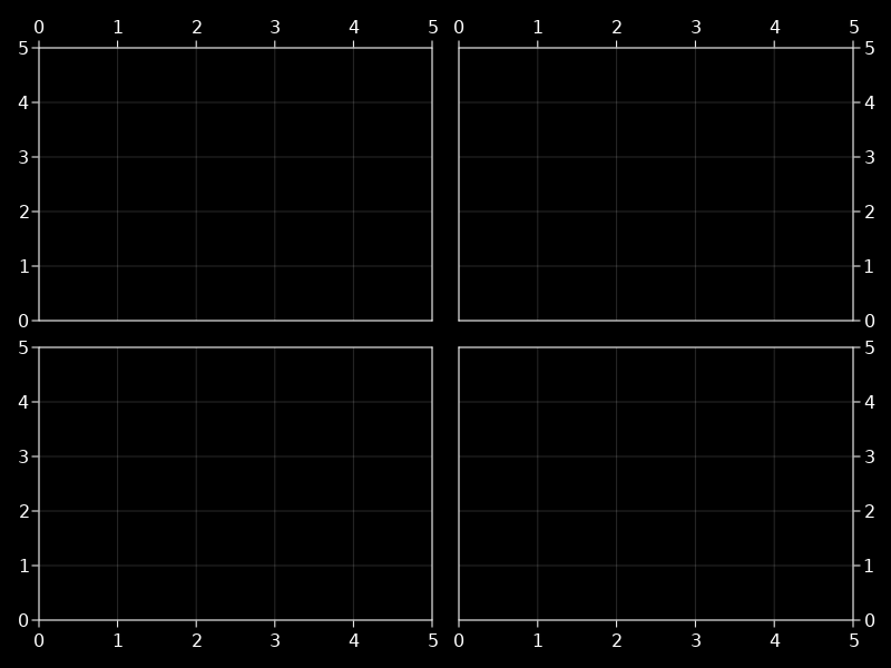
for i in 1:2, j in 1:2
    Axis(
        f[i, j],
        limits = (0, 5, 0, 5),
        xaxisposition = (i == 1 ? :top : :bottom),
        yaxisposition = (j == 1 ? :left : :right))
end

f

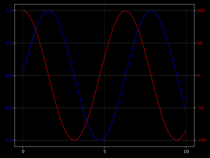
Creating a twin axis

There is currently no dedicated function to do this, but you can simply add an Axis on top of another, then hide everything but the second axis.

Here's an example how to do this with a second y axis on the right.

using CairoMakie

f = Figure()

ax1 = Axis(f[1, 1], yticklabelcolor = :blue)
ax2 = Axis(f[1, 1], yticklabelcolor = :red, yaxisposition = :right)
hidespines!(ax2)
hidexdecorations!(ax2)

lines!(ax1, 0..10, sin, color = :blue)
lines!(ax2, 0..10, x -> 100 * cos(x), color = :red)

f

Axis interaction

An Axis has a couple of predefined interactions enabled.

Scroll zoom

You can zoom in an axis by scrolling in and out. If you press x or y while scrolling, the zoom movement is restricted to that dimension. These keys can be changed with the attributes xzoomkey and yzoomkey. You can also restrict the zoom dimensions all the time by setting the axis attributes xzoomlock or yzoomlock to true.

Drag pan

You can pan around the axis by right-clicking and dragging. If you press x or y while panning, the pan movement is restricted to that dimension. These keys can be changed with the attributes xpankey and ypankey. You can also restrict the pan dimensions all the time by setting the axis attributes xpanlock or ypanlock to true.

Limit reset

You can reset the limits with ctrl + leftclick. This is the same as doing reset_limits!(ax). This sets the limits back to the values stored in ax.limits, and if they are nothing, computes them automatically. If you have previously called limits!, xlims! or ylims!, these settings therefore stay intact when doing a limit reset.

You can alternatively press ctrl + shift + leftclick, which is the same as calling autolimits!(ax). This function ignores previously set limits and computes them all anew given the axis content.

Rectangle selection zoom

Left-click and drag zooms into the selected rectangular area. If you press x or y while panning, only the respective dimension is affected. You can also restrict the selection zoom dimensions all the time by setting the axis attributes xrectzoom or yrectzoom to true.

Custom interactions

The interaction system is an additional abstraction upon Makie's low-level event system to make it easier to quickly create your own interaction patterns.

Registering and deregistering interactions

To register a new interaction, call register_interaction!(ax, name::Symbol, interaction). The interaction argument can be of any type.

To remove an existing interaction completely, call deregister_interaction!(ax, name::Symbol). You can check which interactions are currently active by calling interactions(ax).

Activating and deactivating interactions

Often, you don't want to remove an interaction entirely but only disable it for a moment, then reenable it again. You can use the functions activate_interaction!(ax, name::Symbol) and deactivate_interaction!(ax, name::Symbol) for that.

Function interaction

If interaction is a Function, it should accept two arguments, which correspond to an event and the axis. This function will then be called whenever the axis generates an event.

Here's an example of such a function. Note that we use the special dispatch signature for Functions that allows to use the do-syntax:

register_interaction!(ax, :my_interaction) do event::MouseEvent, axis
    if event.type === MouseEventTypes.leftclick
        println("You clicked on the axis!")
    end
end

As you can see, it's possible to restrict the type parameter of the event argument. Choices are one of MouseEvent, KeysEvent or ScrollEvent if you only want to handle a specific class. Your function can also have multiple methods dealing with each type.

Custom object interaction

The function option is most suitable for interactions that don't involve much state. A more verbose but flexible option is available. For this, you define a new type which typically holds all the state variables you're interested in.

Whenever the axis generates an event, it calls process_interaction(interaction, event, axis) on all stored interactions. By defining process_interaction for specific types of interaction and event, you can create more complex interaction patterns.

Here's an example with simple state handling where we allow left clicks while l is pressed, and right clicks while r is pressed:

mutable struct MyInteraction
    allow_left_click::Bool
    allow_right_click::Bool
end

function MakieLayout.process_interaction(interaction::MyInteraction, event::MouseEvent, axis)
    if interaction.use_left_click && event.type === MouseEventTypes.leftclick
        println("Left click in correct mode")
    end
    if interaction.allow_right_click && event.type === MouseEventTypes.rightclick
        println("Right click in correct mode")
    end
end

function MakieLayout.process_interaction(interaction::MyInteraction, event::KeysEvent, axis)
    interaction.allow_left_click = Keyboard.l in event.keys
    interaction.allow_right_click = Keyboard.r in event.keys
end

register_interaction!(ax, :left_and_right, MyInteraction(false, false))

Setup and cleanup

Some interactions might have more complex state involving plot objects that need to be setup or removed. For those purposes, you can overload the methods registration_setup!(parent, interaction) and deregistration_cleanup!(parent, interaction) which are called during registration and deregistration, respectively.